この記事では、Python言語を用いて、2リンクマニピュレータ(2自由度アーム)の逆運動学を収束計算で求め、シミュレーションする方法をソースコード付きで解説します。
逆運動学の計算(収束計算)
ロボットアームの構造が複雑になると数式で逆運動学が解けなくなります。
そのような場合は、収束計算を用いて解を求めます。
| – | 収束計算の流れ |
|---|---|
| 1 | 仮の解(初期関節角度)を設定する |
| 2 | 仮の解から順運動学を用いて手先位置を求める |
| 3 | 目標位置と手先位置の誤差から仮の解を微修正する |
| 4 | 位置誤差が十分小さくなるまで1~3を繰り返す |
逆運動学の計算プログラム(数値計算)
Pythonを用いて収束計算で逆運動学を解き、姿勢を描画するプログラムを作成しました。
| – | プログラムの処理手順 |
|---|---|
| 1 | 2リンクアームのパラメータ(リンクの長さ、初期関節角度)を設定する |
| 2 | 手先の目標位置を設定する |
| 3 | 逆運動学を収束演算で計算し,目標位置を達成するための関節角度を導出する |
| 4 | 計算結果からアームの姿勢を表示する |
ソースコード
サンプルプログラムのソースコードです。
# -*- coding: utf-8 -*-
import numpy as np
from numpy import sin,cos
import matplotlib.pyplot as plt


# 並進行列(x軸方向に並進)
def L(l):
    Li = np.matrix((
        ( 1., 0., l),
        ( 0., 1., 0.),
        ( 0., 0., 1.)
    ));
    return Li

# 回転行列(z軸周りに回転)
def Rz(th):
    R = np.matrix((
        (cos(th), -sin(th), 0.),
        (sin(th),  cos(th), 0.),
        (0., 0., 1.)
    ))
    return R

# 座標変換行列の微係数(z軸周り)
def dRz(th):
    dR = np.matrix( (
        (-sin(th),-cos(th),0.),
        ( cos(th),-sin(th),0.),
        (0.,0.,0.)
    ));
    return dR

# グラフの描画
def plot(x, y):
    fn = "Times New Roman"
    # グラフ表示の設定
    fig = plt.figure()
    ax = fig.add_subplot(111, axisbg="w")
    ax.tick_params(labelsize=13)                    # 軸のフォントサイズ
    plt.xlabel("$x [m]$", fontsize=20, fontname=fn)
    plt.ylabel("$y [m]$", fontsize=20, fontname=fn)
    plt.plot(x, y,"-g",lw=5,label="link")           # リンクの描画
    plt.plot(x, y,"or",lw=5, ms=10,label="joint")   # 関節の描画
    plt.xlim(-1.2,1.2)
    plt.ylim(-1.2,1.2)
    plt.grid()
    plt.legend(fontsize=20) # 凡例
    plt.show()

def arm2_ik(X, L, th):
    [x, y] = X
    [l1, l2] = L
    [th1, th2] = th
    X = np.matrix(( ( np.array(x) ), ( np.array(y) ) ))
    th1 =  np.radians(th1)  # 仮りの解1
    th2 =  np.radians(th2)  # 仮りの解2

    # 収束計算を50回繰り返す
    for j in range(50):
        # 原点座標(縦ベクトル)
        x = np.array([[0.],[0.],[1.]] )

        P = np.matrix((
            (1.,0.,0.),
            (0.,1.,0.),
            ))

        # 現在の手先位置を求める
        Xg = P * Rz(th1) * L(l1) * Rz(th2) * L(l2) * x

        # ヤコビ行列を求める
        J1 = dRz(th1) * L(l1) * x
        J2 = Rz(th1) * L(l1) * dRz(th2) * L(l2) * x
        JJ = np.c_[J1,J2]                   # 3つの列ベクトルを連結する
        J = P * JJ                            #ヤコビ行列
        invJ = J.T * np.linalg.inv(J * J.T)      #ヤコビ行列の逆行列
        dx = X - Xg             #位置の変位量
        th = 0.1 * invJ * dx      #逆運動学の式
        th1 = th1 + th[0,0]
        th2 = th2 + th[1,0]

    return th1, th2

# 順運動学の計算
def arm2_fk(L, th):
    [l1, l2] = L
    [th1, th2] = th
    vec = np.array([[0.],[0.],[1.]] )
    (x1, y1, z1) = Rz(th1) * L(l1) * vec               # 第1関節の位置
    (x2, y2, z2) = Rz(th1) * L(l1) * Rz(th2) * L(l2) * vec  # 第2関節の位置
    return x1, y1, x2, y2

# メイン
def main():
    # パラメータ
    L = [0.5, 0.5] # リンク1, 2の長さ
    X = [0.5, 0.5] # 手先の目標位置(x,y)
    th = [20, 20]  # 初期関節角度(仮の解)

    # 逆運動学の計算
    th = arm2_ik(X, L, th)

    # 順運動学の計算
    (x1, y1, x2, y2) = arm2_fk(L, th)

    # ロボットアームの描画
    x = (0, x1, x2)
    y = (0, y1, y2)
    plot(x, y)


if __name__ == '__main__':
    main()
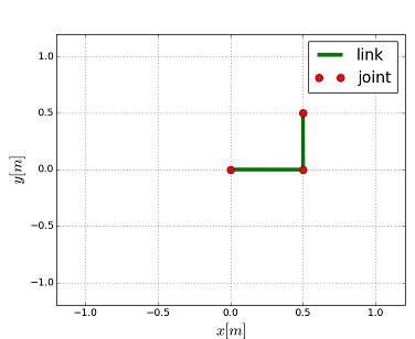
実行結果
サンプルプログラムの実行結果です。
リンク1、2の長さが0.5で手先の目標位置(0.5, 0.5)で計算した結果です。
| – | 関連ページ |
|---|---|
| 1 | ■Pythonでロボットシミュレーション |
| 2 | ■ロボット工学入門 基礎編 |
| 3 | ■Python入門 サンプル集 |
| 4 | ■NumPy入門 サンプル集 |

コメント